|
This tutorial describes how you can use Praat to perform Multi Dimensional Scaling (MDS) analysis.
MDS helps us to represent dissimilarities between objects as distances in a Euclidean space. In effect, the more dissimilar two objects are, the larger the distance between the objects in the Euclidean space should be. The data types in Praat that incorporate these notions are Dissimilarity, Distance and Configuration.
In essence, an MDS-analysis is performed when you select a Dissimilarity object and choose one of the To Configuration (xxx)... commands to obtain a Configuration object. In the above, method (xxx) represents on of the possible multidimensional scaling models.
Let us first create a Dissimilarity object. You can for example create a Dissimilarity object from a file. Here we will the use the Dissimilarity object from the letter R example. We have chosen the default value (32.5) for the (uniform) noise range. Note that this may result in substantial distortions between the dissimilarities and the distances.
Now you can do the following, for example:
Select the Dissimilarity and choose To Configuration (monotone mds)..., and you perform a kruskal-like multidimensional scaling which results in a new Configuration object. (This Configuration could subsequently be used as the starting Configuration for a new MDS-analysis!).
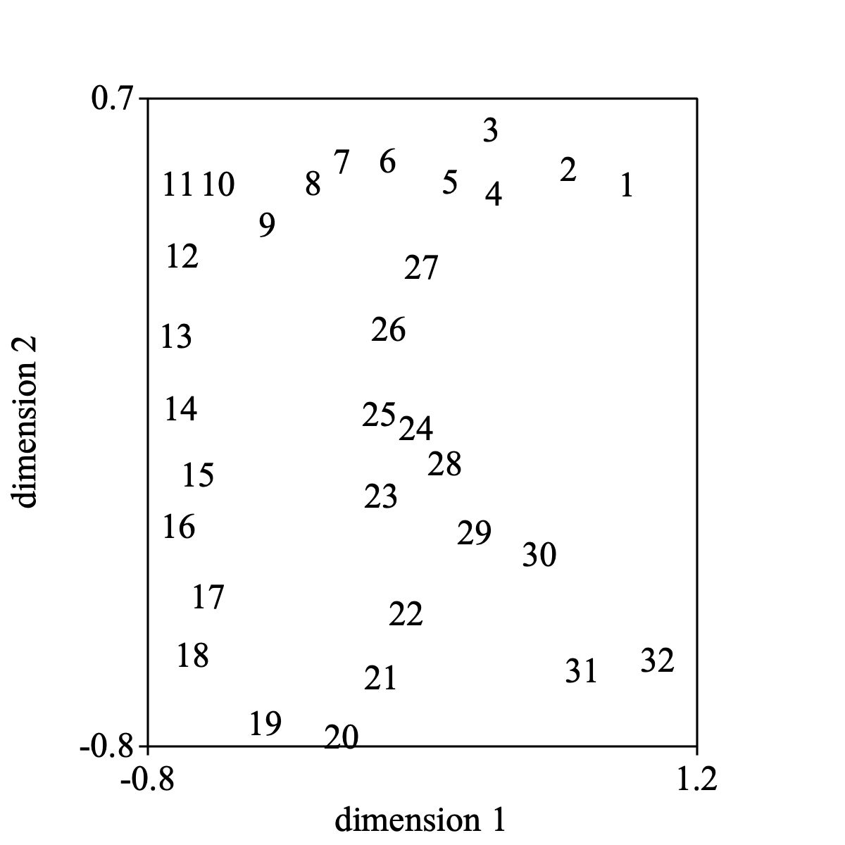
Select the Configuration and choose Draw... and the following picture might result.
The following script summarizes:
dissimilarity = Create letter R example: 32.5
configuration = To Configuration (monotone mds): 2, "Primary approach", 0.00001, 50, 1
Draw: 1, 2, -0.8, 1.2, -0.8, 0.7, "yes"
Select the Dissimilarity and the Configuration together and query for the stress value with: Get stress (monotone mds)....
The following script summarizes:
selectObject: dissimilarity, configuration
Get stress (monotone mds): "Primary approach", "Kruskals's stress-1"
Select the Dissimilarity and the Configuration together to draw the Shepard diagram.
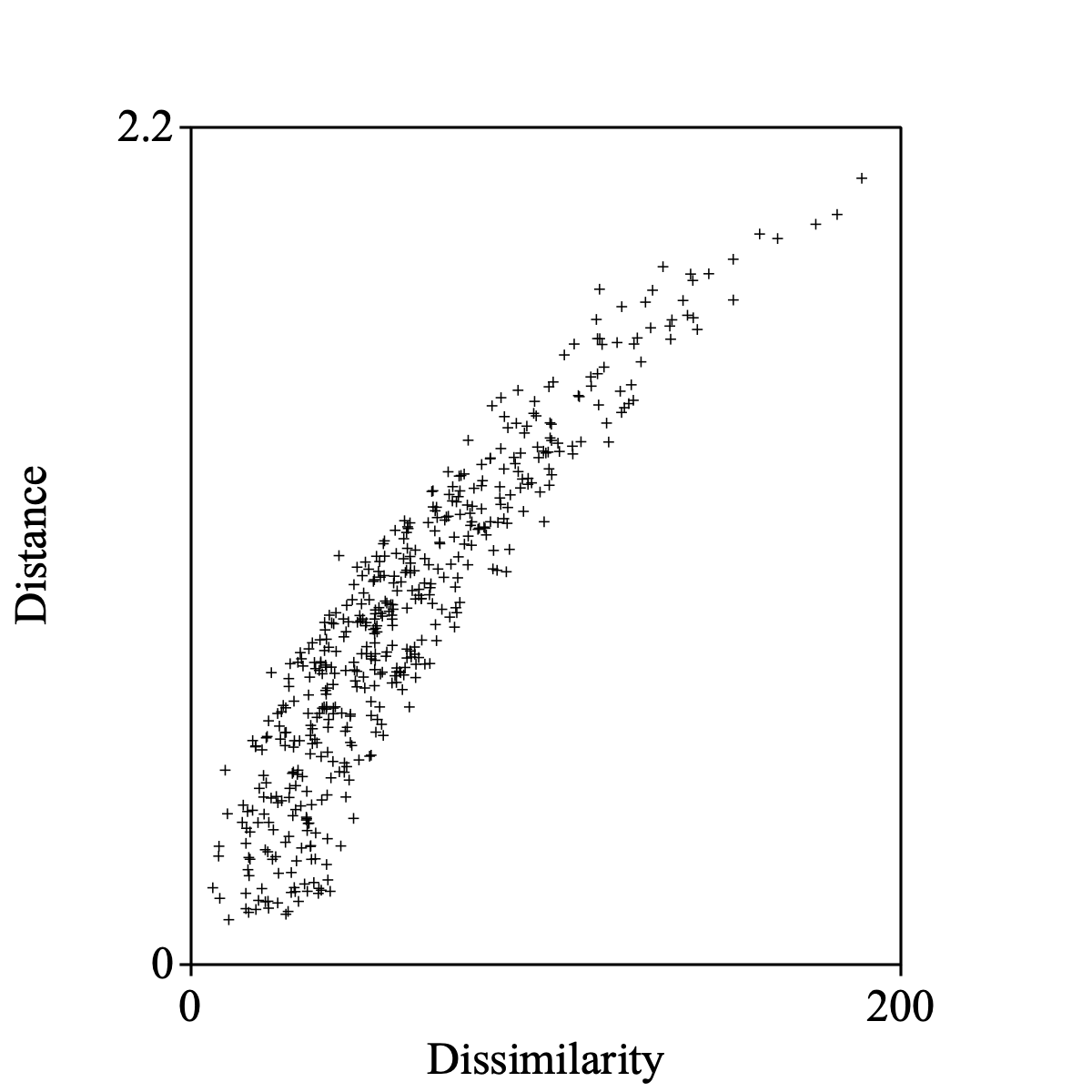
The following script summarizes:
selectObject: dissimilarity, configuration
Draw Shepard diagram: 0, 200, 0, 2.2, 1, "+", "yes"
Select the Dissimilarity and the Configuration together to draw the monotone regression of distances on dissimilarities.
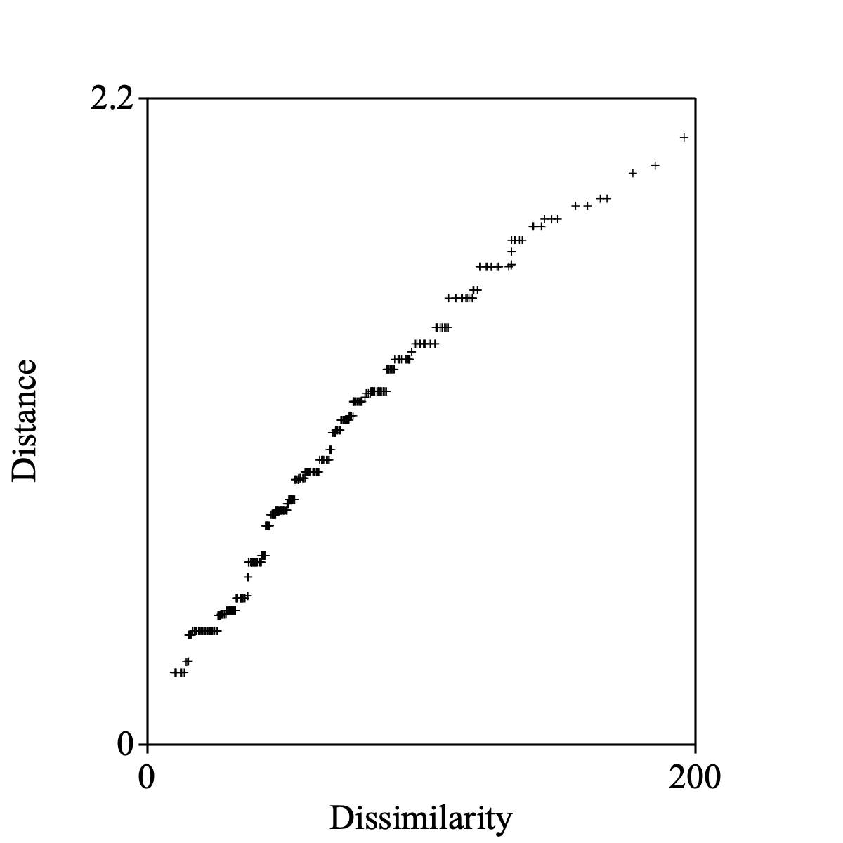
The following script summarizes:
selectObject: dissimilarity, configuration
Draw monotone regression: "Primary approach", 0, 200, 0, 2.2, 1, "+", "yes"
When you enter noiseRange = 0 in the form for the letter R, perfect reconstruction is possible. The Shepard diagram then will show a perfectly smooth monotonically increasing function.
When you can't have equal confidence in all the number in the Dissimilarity object, you can give different weights to these numbers by associating a Weight object with the Dissimilarity object. An easy way to do this is to select the Dissimilarity object and first choose To Weight. Then you might change the individual weights in the Weight object with the Set value... command (remember: make wij = wji).
The following script summarizes:
selectObject: dissimilarity
weight = To Weight
! Change [i] [j] and [j] [i] cells in the Weight object
Set value: i, j, val
Set value: j, i, val
...
! now we can do a weighed analysis.
selectObject: dissimilarity, weight
To Configuration (monotone mds): 2, "Primary approach", 0.00001, 50, 1)
You can also query the stress values with three objects selected. The following script summarizes:
selectObject: dissimilarity, weight, configuration
Get stress (monotone mds): "Primary approach", "Kruskals's stress-1"
You could also use a Configuration object as a starting configuration in the minimization process. Let's assume that you are not satisfied with the stress value from the Configuration object that you obtained in the previous analysis. You can than use this Configuration object as a starting point for further analysis:
The following script summarizes:
selectObject: dissimilarity, configuration, weight
To Configuration (monotone mds): 2, "Primary approach", 0.00001, 50, 1
When you have multiple Dissimilarity objects you can also perform individual difference scaling (often called INDSCAL analysis).
As an example we can use an example taken from Carrol & Wish. Because INDSCAL only works on metrical data, we cannot use Dissimilarity objects directly. We have to transform them first to Distance objects.
This type of analysis on multiple objects results in two new objects: a Configuration and a Salience.
© djmw 20140117