|
Multidimensional scaling (MDS) models are defined by specifying how given Dissimilarity data, δij, are mapped into distances of an m-dimensional MDS Configuration X. The mapping is specified by a representation function, f : δij → dij(X), which specifies how dissimilarities should be related to the distances. The MDS analysis tries to find the configuration (in a given dimensionality) whose distances satisfy f as closely as possible. This closeness is quantified by a badness-of-fit measure which is often called stress.
In the application of MDS we try to find a configuration X such that the following relations are satisfied as well as possible:
| f(δij) ≈ dij(X) |
The numbers that result from applying f on δij are sometimes called disparities d′ij. In most applications of MDS, besides the configuration X, also the function f is not completely specified, i.e., the exact parameters of f are unknown and must also be estimated during the analysis. If no particular f can be derived from a theoretical model, one often restricts f to a particular class of functions on the basis of the scale level of the dissimilarity data. If the disparities are related to the proximities by a specific parametric function we speak of metric MDS otherwise we speak of ordinal or non-metric MDS.
| if δij < δkl, then dij(X) < dkl(X) |
More information on all aspects of multidimensional scaling can be found in: Borg & Groenen (1997) and Ramsay (1988).
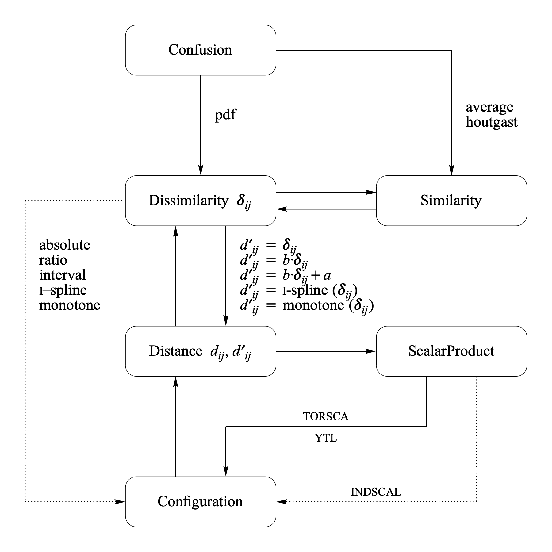
The most important object types used in Praat for MDS and the conversions between these types are shown in the following figure.
© djmw 20101109